Having spent quite a lot of time on another code project, it’s high time I got back to a little tafl.
Remember where we left off: board states represented as arrays of small integers, and taflman objects inflated as needed during game tree search. It turns out that inflating and deflating taflmen is also a potential source of slowness, so I went ahead and removed that code from the game. (It also greatly simplifies the process of moving from turn to turn.) Wherever I would pass around the old taflman object, I now pass around a character data type, the sixteen bits I described in the previous tafl post.
This revealed two further slowdowns I had to tackle. The first, and most obvious, was the algorithm for detecting encirclements. For some time, I’ve known I would need to fix it, but I didn’t have any ideas until a few weeks ago. Let’s start with the old way:
 for each potentially-surrounded taflman:
   get all possible destinations for taflman
     for each destination:
     if destination is edge, return true
 return false
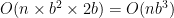
Simple, but slow. In the worst-case scenario, each taflman has to consider every other space on the board, and look briefly at every other space from each rank and file (where n is the number of taflmen and b is the board dimension):
I was able to cut this down some by running an imperfect fast check: if, on any rank or file, the allegedly-surrounded side has the taflman nearest either edge, that side is not surrounded. That had implications for a better algorithm, and sure enough, I hit on one.
 list spaces-to-explore := get-all-edge-spaces
 list spaces-considered := []
 for space in spaces-to-explore:
   add space to spaces-considered
   get neighbors for space not in spaces-to-explore and not in spaces-considered
   for each neighbor:
     if neighbor is occupied:
       if occupier belongs to surrounded-side:
         return false
       else continue
     else:
       add neighbor to spaces-to-explore
 return true
More complicated to express in its entirety, but no more difficult to explain conceptually: flow in from the outside of the board. Taflmen belonging to the surrounding side stop the flow. If the flow reaches any taflman belonging to the allegedly surrounded side, then the allegedly surrounded side is, indeed, not surrounded. This evaluation runs in a much better amount of time:

Astute readers might note that, since the board dimension is never any larger than 19 at the worst, the difference between a square and a cube in the worst-case runtime isn’t all that vast. Remember, though, that we need to check to see whether every generated node is an encirclement victory, since an encirclement victory is ephemeral—the next move might change it. Running a slightly less efficient search several hundred thousand to several million times is not good for performance.
I found another pain point in the new taflman representation. The new, array-based board representation is the canonical representation of a state, so to find a taflman in that state, the most obvious move is to look through the whole board for a taflman matching the right description. Same deal as with encirclement detection—a small difference in absolute speed makes for a huge difference in overall time over (in this case) a few tens of millions of invocations. I fixed this with a hash table, which maps the 16-bit representation of a taflman to its location on the board. The position table is updated as taflmen move, or are captured, and copied from state to state so that it need be created only once. Hashing unique numbers (as taflmen representations are) is altogether trivial, and Java’s standard HashMap type provides a method for accessing not only the value for a given key, but also a set of keys and a set of values. The set of keys is particularly useful. Since it’s a canonical list of the taflmen present in the game, it saves a good bit of time against looping over the whole of the board when I need to filter the list of taflmen in some way.
Those are all small potatoes, though, next to some major algorithmic improvements. When we last left OpenTafl, the search algorithm was straight minimax: that is, the attacking player is the ‘max’ player, looking for board states with positive evaluations, and the defending player is the ‘min’ player, looking for the opposite. Minimax searches the entire game tree.
Let’s look at an example, a tree of depth 3 with max to play and a branching factor of 3, for 9 leaf nodes. The leaf nodes have values of 7, 8, and 9; 4, 5, and 6; and 12, 2, and 3. We can express the minimax perspective on this tree mathematically:

That is to say, max makes the move which gives min the least good best response. Remember, though, that we search the tree depth-first, which means that in the formula above, we move from left to right. This leaves us with some room for cleverness.
Consider this:

Does it matter what the numbers at x, y, and z are? No: by that time, we’ve already established that the subtrees in which they appear (with best possible values 4 and 2) are worse than the first subtree (with known value 7). Therefore, we can stop exploring those subtrees. This is known as ‘pruning’.
Pruning is good, because, when done correctly, it saves us work without dropping good moves. Alpha-beta pruning, the kind described above, is known to produce identical results to minimax, and, in the ideal case, can search twice as deep. (So far, it’s only given me one extra ply, though; the case isn’t quite ideal enough for more.) Other kinds of pruning may find their way in later, and will take some more careful thinking to avoid pruning away potentially good branches.
What is the ideal case, then? We want to explore the best moves first. A cursory examination of the example case above provides the reasoning. If we explore the subtrees in opposite order, we can do no pruning, and we get no speedup. This presents us with a chicken-and-egg problem: if we could easily and programmatically determine which moves are good, we wouldn’t need to bother with variants on full-tree search at all.
Fortunately, the structure of a tree gives us an easy out. Most of the nodes in any given tree are at the bottom. Consider a simple example, with a branching factor of two. At the first level, there’s one node; at the next, two nodes; at the third, four nodes; and at the fourth, eight nodes. In every case, there are more nodes at the deepest level than at all the levels above combined. The difference becomes more pronounced with greater branching factors: a tree with a branching factor of 30 (which approximates brandub) has a distribution of 1/30/900/27,000. So, it follows that the large majority of the work in a game tree is expanding the game states at the target search depth, and evaluating those states; the work higher up the tree is almost trivial.
Take that and add it to this claim: the best move at any given depth is likely to have been one of the best moves at the immediately prior depth, too. We can use those facts together to figure out the best ordering for our moves at our target depth: search to the depth prior, keep track of the best moves at that depth, and search them first. This approach is called ‘iterative deepening’: generally, you start at depth 1, and use results from previous levels to order each node’s children. OpenTafl accomplishes this with a structure I’m calling a deepening table, which is generated for each . The deepening table is a list of maps, one per depth. The maps relate a position hash to an evaluation done at its depth. On each deepening iteration, the exploration function generates successor states, then sorts them according to the data stored in the deepening table before exploring further. (There’s some easy performance on the table here—since creating a full-on successor state is a non-trivial operation, I can probably buy myself some easy speedup by generating moves alone, sorting those based on the positional hashes which would result from making those moves, and only generating states immediately before exploring them. This would probably save a good bit of time by never generating states which would have otherwise been cut off by alpha-beta pruning.)
Implementing the deepening tables put me on the scent of another major optimization, the transposition table. A transposition table stores values for previously-visited states, along with the depth each state was previously searched to. (If we’re searching six plies deep and previously encountered a state at depth four, that state was only searched to a depth of two. If we encounter the same state at depth two, then if we use the cached value, we’ve left two plies of depth on the table.) Hits in the transposition table early on in the search save us expanding whole subtrees, which yields many fewer node expansions required per search, and lets us reach deeper more easily.
The transposition table, since it persists through the entire game, must be limited in size by some mechanism. OpenTafl’s transposition table is an array of Entry objects, with a fixed size in megabytes. The array is indexed by positional hashes, modulo the size of the table. When indices collide, OpenTafl decides whether to replace the old value based on its age (older values are more readily discarded) and the depth to which it is searched (deeper searches are kept, if both are equally as fresh).
That brings me to the end of another marathon tafl post. Stay tuned for another one—probably a much shorter one—in the not-too-distant future, as I wrap up work on this sprint of OpenTafl, with an eye toward the first public code and source release.